Retrieving Sources and Lightcurves from the IRSA Databases
The source and lightcurve databases are new deliverables for PTF/iPTF and are included in DR3. A summary of the lightcurve construction process and content was given here. Below we give instructions on how to access and query the lightcurve database table.
Access
The source and lightcurve database tables can be accessed as follows:
- Go to: http://irsa.ipac.caltech.edu.
- Click on the "Catalogs" icon.
- Choose the "PTF" radio button and click "Select" at the top.
- You will be taken to a page that shows:
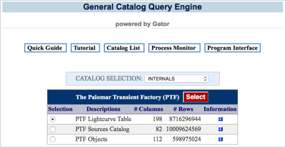
You can select from one of three tables:
PTF Objects - the targets that label each individual lightcurve with "collapsed-lightcurve" metrics. For objects with transient_flag = 0, the object is tied to a reference-image (coadd) detection. If so, metadata characterizing the extracted reference-image source is also given. Such objects may be associated with time-variable sources that "survived" the co-addition process. For objects with transient_flag = 1, the object is transient at one or more epochs and would have been flagged as an outlier (hence omitted) during co-addition. If so, no associated reference-image metadata exists, although collapsed-lightcurve metrics are still given. Expanded descriptions of each column in this table are available.
PTF Sources Catalog - table containing all the epoch-based source photometry and metadata extracted from the epochal images (SExtractor-based), specifically to support lightcurve construction for DR3. Note: not all the epochal data currently available in the image/catalog archive is loaded [see Scope and Content for DR3].
PTF Lightcurve Table - table view that contains the individual lightcurves, i.e., that associates each object (target) in the Objects Table to all epochal apparitions (detections) of that object in the Sources Catalog. The Lightcurve Table combines all columns and metadata from both the Objects and Sources Catalog tables. Expanded descriptions of each column in this table are also available.
Each of the above tables can be independently queried. The table you're most likely to query is the Lightcurve Table. Below we focus on use cases for querying this table. The same underlying query engine and functionality applies to the other tables.
Use case 1 (Lightcurve table): single object searches
You can supply a single position (e.g., ra dec = 312.333629 -1.078686 falls on a known RR-Lyrae variable) and either a search radius (<= 30 arcsec) or a box size (<= 60 arcsec) centered on this position. All objects and their lightcurves falling inside this search region will be returned after clicking "Run Query" (see below). You can narrow down this search region to better localize your target (i.e., <~ 3 arcsec to account for astrometric uncertainty). The names of known objects can also be specified in this search box.
The columns at the bottom are those that will be returned by default (the "Standard" table). These are pre-selected for you (using the blue checkboxes). There is also a "Long Form" that lists additional lightcurve metrics. The latter are not pre-selected since there are many of them. Use the checkboxes to select/de-select any columns. You can also specify filtering constraints in the dialogue boxes beside each column. A popular one is forcing fid=1 (g filter) or fid=2 (R filter).
Clicking "Run Query" will submit the query and display the results on your browser. An image showing your target position (cross) and the positions of all your returned objects falling in your search region is presented at the top. There are pull-down menus to change the overlay image (e.g., 2MASS, SDSS, WISE, ...). At this time, PTF images from the archive cannot be selected. This will be enabled in future. Beside this image is a simple lightcurve plot of mag_autocorr (= refined absolute photometry) versus obsmjd from the table at the bottom. This plot panel also has menus for zooming or selecting specific points. Selecting a specific point will highlight the corresponding table row at the bottom.
The returned table at the bottom can be further filtered on a per-column basis, for example, if lightcurves for multiple objects were returned, you can retain specific objects of interest by clicking on the funnel icon under the oid (object ID) column.
NOTE: the format/structure of the returned table is such that all lightcurve-collapsed metrics/metadata associated with each unique object are repeated at each epoch (obsmjd), while epoch-dependent metrics (i.e., mag_autocorr, fwhm, ...) will vary, obviously. This table can be saved to ASCII (IPAC-table) format for massaging offline by clicking on "Result IPAC Table".
"To Periodogram" button: this sends the entire table to a periodogram service; before it does however, a new page will open presenting you with which objects (oid's) you would like a periodogram. After selecting your oid of interest, a periodogram is computed together with period estimates and phased lightcurves for each candidate period.
Use Case 2 (Lightcurve table): polygon search
To query a larger search region (e.g., the boundaries of a specific PTF field or CCD image), you can use the "Polygon" search feature on the query panel. Beware that polygons spanning large regions, typically several degrees or more, will take longer to process. An example format specification for the polygon vertices is given here.
The same functionality and format described under "Use Case 1" above will apply to the output results from a polygon search. The only difference is that more object lightcurves will be returned.
Use Case 3 (Lightcurve table): muiti-object search
This can be selected by checking the "Multi-Object Search" radio button at the top of the query page. This enables you to upload a table of target positions and search-area constraints for each. Here's an example upload file you can experiment with. The column labelled "major" is interpreted as a search radius. Example specifications for other search-region options are given here.
Selecting "One-to-One Match" on the query panel will filter the output results such that the closest matching object to each input position is reported, if found within the search region. If not found, the returned rows are filled with "null" so that a one-to-one correspondence with the input list is retained. If "One-to-One Match" is not selected, then potentially multiple objects (and their lightcurves) falling in each search region will be returned. The "One-to-One Match" option is therefore convenient for filtering unwanted objects, provided you have a good handle on the positional uncertainties, although beware in regions with a high source-density. The closest match may not be the correct one.
The same functionality and format described under "Use Case 1" above will apply to the output results from a multi-object search.
Use Case 4 (Lightcurve table): all-sky search
This option can also be selected at the top of the query page. This option does not return lightcurves. Its purpose is to obtain counts from the entire database table, subject to any column-constriants specified in the table at the bottom.